
Autoregressive Integrated Moving Average (ARIMA) models have long been a staple in the world of financial forecasting, offering a nuanced approach to predicting future market trends based on past data. With the advent and proliferation of cryptocurrency markets, the application of ARIMA time series models has found new relevance, providing traders and investors with a sophisticated tool to navigate the notoriously volatile crypto terrain.
At its core, the ARIMA model leverages time series data to understand and forecast market movements. This involves analyzing patterns within the data, such as trends and seasonality, and using these insights to make educated predictions about future prices. The model is particularly suited to crypto markets due to their rapid fluctuations and the wealth of available trading data.
In this blog article, we delve into the fundamentals of ARIMA models and explore their application in the context of cryptocurrency markets. We’ll discuss how these models work, the process of fitting an ARIMA model to crypto market data, and the potential benefits and limitations of using ARIMA for crypto market forecasting. Whether you’re a seasoned trader or new to the world of cryptocurrency, understanding how ARIMA models can be used for market forecasting is an invaluable tool in your trading arsenal.
What are ARIMA Time Series Models?
ARIMA models, short for Autoregressive Integrated Moving Average, are a class of statistical models used for analyzing and forecasting time series data. These models are particularly adept at capturing various patterns in sequential data sets, making them invaluable for financial market forecasting, including the volatile cryptocurrency markets. An ARIMA model is defined by three key parameters: p, d, and q.
- Autoregressive (AR) component (p): This aspect of the model captures the relationship between an observation and a specified number of lagged observations. The parameter p represents the order of the autoregressive part, indicating the number of lagged terms of the series that are used as predictors.
- Integrated (I) component (d): Integration involves differencing the time series data d times to make it stationary, meaning the data’s statistical properties, such as mean and variance, do not change over time. Stationarity is crucial for the predictive accuracy of ARIMA models, as it ensures that the model’s parameters remain constant over time.
- Moving Average (MA) component (q): The MA part models the relationship between an observation and a residual error from a moving average model applied to lagged observations. The parameter q specifies the order of the moving average component, or the number of lagged forecast errors that the model includes.
The synergy of these components allows ARIMA models to efficiently handle data with trends, seasonality, and other complex patterns, making them a powerful tool for time series analysis. The selection of p, d, and q parameters is crucial, as it directly influences the model’s ability to capture the underlying patterns in the data accurately. Understanding and correctly identifying these parameters can significantly enhance the model’s forecasting performance.
The Mathematics Under The Hood
The ARIMA (Autoregressive Integrated Moving Average) model is a comprehensive tool for analyzing and forecasting time series data, integrating the Autoregressive (AR) process, differencing (I – Integrated), and the Moving Average (MA) process. The model is denoted as ARIMA(p, d, q), where:
- p represents the order of the Autoregressive terms
- d indicates the degree of differencing required to make the series stationary
- q denotes the order of the Moving Average terms.
The formula for an ARIMA model can be dissected into three main components:
Integrated (I) Component: This involves differencing the time series data d times to achieve stationarity. Stationarity implies that the statistical properties of the series do not change over time. The differencing operation is represented as:
[math]Y’_t = (1 – B)^d Y_t[/math]
Here, Yt is the original series, Yt′ is the differenced series, B is the backshift operator, and d is the degree of differencing.
Autoregressive (AR) Component: The AR part models the differenced series as a linear function of its previous values. For an AR order of p, the expression is:
[math]\phi(B)Y’_t = \phi_1 Y’_{t-1} + \phi_2 Y’_{t-2} + … + \phi_p Y’_{t-p}[/math]
ϕ1,ϕ2,…,ϕp are the coefficients of the model, and ϕ(B) represents the AR polynomial involving the backshift operator B.
Moving Average (MA) Component: This component models the error term as a linear combination of error terms from previous time points. For a MA order of q, the formula is:
[math]\theta(B)\epsilon_t = \theta_1 \epsilon_{t-1} + \theta_2 \epsilon_{t-2} + … + \theta_q \epsilon_{t-q}[/math]
Here, θ1,θ2,…,θq are the MA coefficients, and θ(B) signifies the MA polynomial with the backshift operator B.
The combined ARIMA model formula, integrating the differencing, AR, and MA components, is given by:
[math]\phi(B)(1 – B)^d Y_t = \theta(B)\epsilon_t[/math]
The 3 terms we just described are part of the expression of the derivative of the time series we want to predict:
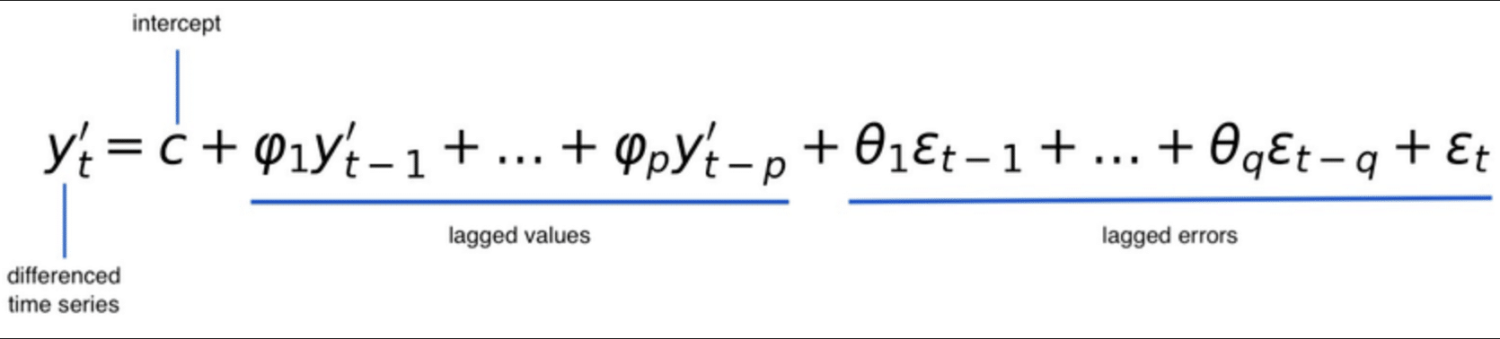
This equation succinctly captures the essence of the ARIMA model, showing how it employs differencing to stabilize the time series, uses AR terms to account for autocorrelations, and incorporates MA terms to handle noise or error components, making it a robust framework for time series analysis and forecasting.
How are they Used for Markets Forecasting?
ARIMA models have long been a cornerstone in the field of financial market forecasting, offering a systematic and quantitative approach to predicting market trends. Traditionally, these models have been applied to stock markets, commodities, and economic indicators, where they analyze historical data to forecast future values. The strength of ARIMA models lies in their ability to model a wide range of time series data, capturing the underlying patterns of autocorrelation and trends within the financial markets.
The transition of ARIMA models’ application from traditional financial markets to cryptocurrency markets represents a significant expansion in their use. Cryptocurrency markets, known for their high volatility and unpredictability, present unique challenges and opportunities for time series analysis. ARIMA models are particularly suited to these markets due to their flexibility in modeling non-stationary data, which is a common characteristic of cryptocurrency price movements. By differencing the data to achieve stationarity and using the autoregressive and moving average components to account for market dynamics, ARIMA models can effectively forecast cryptocurrency prices.
The benefits of using ARIMA models for market forecasting are manifold. Firstly, they provide a structured approach to understanding market trends, allowing analysts to quantify and predict future movements based on historical data. This is invaluable in making informed trading and investment decisions. Secondly, ARIMA models can be tailored to the specific characteristics of a financial market, including the volatile nature of cryptocurrencies, by adjusting their parameters (p, d, q) to best fit the observed data. Lastly, the ability of ARIMA models to incorporate seasonal patterns and trends means they can adapt to the ever-changing dynamics of financial markets, offering forecasts that are both relevant and timely.
An Example of Implementation in Python for BTC
Implementing an ARIMA model for Bitcoin (BTC) price forecasting involves several steps, including data collection, model fitting, and prediction. Below is a simplified example using Python. This example assumes you have historical Bitcoin price data available in a CSV file and will use the pandas library for data manipulation and the statsmodels library for ARIMA modeling.
Step 1: Import Libraries
import pandas as pd
import numpy as np
from statsmodels.tsa.arima.model import ARIMA
import matplotlib.pyplot as plt
Step 2: Load and Prepare the Data
# Load the dataset
df = pd.read_csv('path_to_your_BTC_price_data.csv')

# Assume the CSV has columns 'Date' and 'Close' for closing prices
df['Date'] = pd.to_datetime(df['Date'])
df.set_index('Date', inplace=True)

# Use closing price as the series
btc_prices = df['Close']
Step 3: Visualize the Data
btc_prices.plot(title='BTC Closing Prices')
plt.show()
Step 4: Fit the ARIMA Model
Before fitting the model, you should perform a stationarity test (e.g., ADF test) and determine the (p,d,q) parameters. This example will use placeholder values for (p,d,q).
# Fit the ARIMA model
# Note: (p,d,q) should be chosen based on data analysis
model = ARIMA(btc_prices, order=(5,1,0))  # Example: ARIMA(5,1,0)
model_fit = model.fit()

# Summary of the model
print(model_fit.summary())
Step 5: Make Predictions
# Forecast the next 5 days
forecast = model_fit.forecast(steps=5)

# Print the forecast
print(forecast)
Step 6: Plot the Results
# Plot the past closing prices along with the forecast
plt.figure(figsize=(10,6))
plt.plot(btc_prices.index, btc_prices, label='Historic BTC Prices')
plt.plot(forecast.index, forecast, color='red', label='Forecasted Prices')
plt.legend()
plt.show()