The Bellman-Ford Algorithm

Have you ever found yourself lost in a city, desperately in need of directions? In the realm of computers, there’s an algorithm that tackles this very predicament. Introducing the Bellman-Ford algorithm, a graph search strategy that has shaped the digital landscape in more ways than one. What is the Bellman-Ford algorithm?

The Bellman-Ford algorithm is named after Richard Bellman and Lester Ford, Jr., who independently developed it in the mid-20th century. This algorithm represents a cornerstone in the world of computer science and operations research, finding wide applicability in diverse fields, from telecommunications and computer networking, to air travel and logistics. It serves as a robust solution for one of the most fundamental problems in graph theory: finding the shortest path between two nodes.

At its core, the Bellman-Ford algorithm is a single-source shortest path algorithm, capable of handling graphs with negative weight edges—an area where its famous counterpart, Dijkstra’s algorithm, falls short. Although it’s a bit slower compared to Dijkstra’s, Bellman-Ford makes up for it with its versatility, enabling solutions for a wider range of problems. It’s a classic example of a dynamic programming algorithm, highlighting the power of breaking a large problem into smaller, more manageable sub-problems.

The Bellman-Ford algorithm’s most remarkable feature, perhaps, is its ability to detect negative cycles within a graph. Negative cycles can wreak havoc in many applications, distorting the path length between nodes. By identifying these problematic elements, the algorithm prevents the propagation of inaccurate or misleading data.

This article aims to provide a comprehensive understanding of the Bellman-Ford algorithm.

Bellman-Ford Algorithm Pseudocode Explained

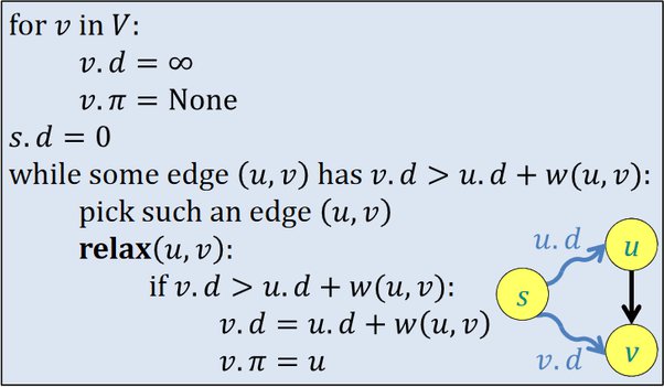
let’s begin with a simplified pseudocode of the Bellman-Ford algorithm, followed by a detailed breakdown of the steps involved. This pseudocode assumes we are given a weighted directed graph with n nodes, an array of edges edge[] where each edge contains the source, destination, and weight, and a source node src.

function BellmanFord(graph, src):
    Initialize distance array dist[] = Infinite for all vertices, except dist[src] = 0

    for i from 1 to size(vertices)-1:
        for each edge(u, v, w) in edge[]:
            if dist[u] + w < dist[v]:
                dist[v] = dist[u] + w

    for each edge(u, v, w) in edge[]:
        if dist[u] + w < dist[v]:
            print "Graph contains a negative-weight cycle"

    print "Shortest distances from source:"
    for each vertex v:
        print "Vertex:", v, " Distance:", dist[v]

Let’s break down this pseudocode into steps:

1. Initialization: Start by initializing an array of distances. Set the distance to all nodes as infinite, except for the source node, which should be set to 0. This is because the distance from the source to itself is always 0.
2. Relaxing the edges: Relax all the edges n-1 times, where n is the number of vertices in the graph. For each edge (u, v) with weight w, if the distance to u plus the weight of the edge (u, v) is less than the current known distance to v, update the distance to v. This is done because we’ve found a shorter path to v through u.
3. Checking for negative-weight cycles: Once the distances to all vertices have been finalized, perform one more pass over all the edges. If you can still update a distance, then there is a negative-weight cycle in the graph. This is because a shorter path should not exist once all the distances are finalized unless the path leads through a negative cycle.
4. Output: Finally, print the shortest distances from the source node to all other nodes.

This algorithm works based on the principle of dynamic programming, breaking down the problem into smaller overlapping sub-problems and building up an optimal solution. It ensures that every shortest path in the graph is found, accounting for the possibility of negative weight edges and cycles.

Bellman-Ford Algorithm: a Python Implementation

Here is a Python implementation of the Bellman-Ford Algorithm. This program assumes that the input graph is represented by an adjacency list.

class Graph:
    def __init__(self, vertices):
        self.V = vertices
        self.graph = []

    def add_edge(self, u, v, w):
        self.graph.append([u, v, w])

    def print_solution(self, dist):
        print("Vertex Distance from Source")
        for i in range(len(dist)):
            print("{0}\t\t{1}".format(i, dist[i]))

    def bellman_ford(self, src):
        dist = [float("Inf")] * self.V
        dist[src] = 0

        for _ in range(self.V - 1):
            for u, v, w in self.graph:
                if dist[u] != float("Inf") and dist[u] + w < dist[v]:
                    dist[v] = dist[u] + w

        for u, v, w in self.graph:
            if dist[u] != float("Inf") and dist[u] + w < dist[v]:
                print("Graph contains negative weight cycle")
                return

        self.print_solution(dist)

# Usage
g = Graph(5)
g.add_edge(0, 1, -1)
g.add_edge(0, 2, 4)
g.add_edge(1, 2, 3)
g.add_edge(1, 3, 2)
g.add_edge(1, 4, 2)
g.add_edge(3, 2, 5)
g.add_edge(3, 1, 1)
g.add_edge(4, 3, -3)

g.bellman_ford(0)

In the given Python program:

• The Graph class represents the directed graph. Each graph object has a list of edges (self.graph), and self.V represents the number of vertices in the graph.
• The add_edge method appends an edge to the graph.
• The bellman_ford method implements the core of the Bellman-Ford algorithm. It starts by initializing the distance from the source to all other vertices as Infinity, except the distance from the source to itself, which is 0. It then relaxes all the edges V-1 times and checks for negative-weight cycles.
• The print_solution method prints the shortest path from the source to all other vertices.

Please note that this algorithm does not account for unreachable vertices, so you might need to make modifications if your use case involves such scenarios.

Conclusion

The algorithm’s versatility, enabled by its ability to handle negative weights and detect negative cycles, sets it apart from other shortest path algorithms. While it may not be the fastest, its comprehensive applicability and dynamic programming nature demonstrate a striking balance between speed and utility.

Moreover, studying the Bellman-Ford algorithm provides invaluable lessons in problem-solving, particularly the concept of breaking down larger problems into more manageable subproblems. The implementation of this algorithm serves as an excellent practical example of dynamic programming, an essential technique in the toolbox of any aspiring computer scientist.

Finally, as we push forward into an era where the complexity and interconnectivity of systems continue to grow, the relevance and application of the Bellman-Ford algorithm are expected to expand. Its fundamental principles continue to inspire new algorithms and strategies in graph theory and beyond.

In conclusion, the Bellman-Ford algorithm is not just a part of computer science’s history; it’s a vital tool for the present and an inspiration for future algorithms. Its robustness, adaptability, and utility render it a powerful beacon in the landscape of algorithmic problem-solving, underscoring the elegance and impact of computer science on our everyday lives.