
Neural networks power a wide range of deep learning applications in different industries with different use cases, from natural language processing (NLP) to computer vision.
But when dealing with sequential or time-series data, traditional neural networks cannot be used for learning and prediction. A mechanism is needed to retain past or historical data to predict future values. Recurrent Neural Networks or RNNs for short are a variant of artificial neural networks that can process sequential data and can be trained to hold knowledge of the past. RNNs are commonly used in the fields of machine learning, natural language processing and pattern recognition.
In this article, we will introduce recurrent neural networks and their architecture, the types of Deep Learning models based on RNNs and examples of models based on this type of network.
What is a recurrent neural network?
RNNs are ideal for solving problems where the sequence is more important than individual elements themselves. They are generally used to treat sequential datawhich can be time series data or text data in any format.
Sequences are objects each element of which has an order, a position, an inscription in time. For example, in a sentence, each word comes in a certain order and it is pronounced on a separate time interval from that of the others.
Due to their internal memory, RNNs can remember important things about the input they received, allowing them to be very accurate in predicting what comes next. In a standard neural network, information only moves in one direction, from the input layer, through the hidden layers, to the output layer. Information flows directly through the network and never touches a node twice.
In an RNN, the information goes through a loop. When making a decision, it considers current data and what it has learned from previously received data.

Let’s imagine we have a classical neural network and give it the word Bonjour as input and it processes the word character by character. By the time it reaches the character jhe has already forgotten b, o And nmaking it almost impossible for this type of neural network to predict which letter would come next.
An RNN, however, is able to remember these characters due to its internal memory. It produces output, copy and loop in the network.
To get more layers of computation to be able to solve or estimate more complex tasks, the output of the RNN could be fed into another RNN, or any number of layers of RNNs.
Architecture of an RNN
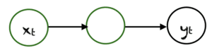
Consider the forward propagation single neural unit or feedforward this below on the right. This unit has a single hidden layer. ${X}{t}$ is its input and ${Y}{t}$ is its output at a specific time t. If we want to create a simple recurring unit from it, then all we need to do is create a connection back from the hidden layer to itself to access the information of time t-1. This feedback loop involves a delay of one unit time. So one of the entries of ${H}{t}$ is ${H}{t-1}$, in turn the hidden layer has two inputs each time, its current value and its own last value. In summary, this feedback loop allows information to flow from one stage of the network to another and thus acts as memory in the network.

The diagram below illustrates the architecture with the weights:

From the figure above, we can write the equations below:
$$ \left{\begin{matrix} \mathbf{H}t = \phi(\mathbf{X}t \mathbf{W}{x} + \mathbf{H}{t-1} \mathbf{W}_{h} + \mathbf{b}h) \ \mathbf{O}t= \mathbf{H}{t} \mathbf{W}{o} + \mathbf{b}_t \end{matrix}\right. $$
- The quantity ${Y}_{t}$ is the output of the recurrence layer at t. This is therefore a vector of size h.
- The ${H} state{t}$ which is not used by output, but which will be used in the calculation for the next date. This is also the reason why we assign the hidden state name, because ${H}{t}$ is only used for computation and does not output from the layer neurons.
- ${W}_{x}$ the input weights of the recursive layer.
- ${W}_{h}$ the weights inside the neurons for the hidden state.
- ${W}_{0}$ the output weights of the recursive layer.
At iteration t, we calculate ${H}{t}$ by involving the hidden state of the previous iteration ${H}{t-1}$ and current input ${X}{t}$ from the weights, to then calculate the output ${Y}{t}$. The current hidden state ${H}_{t}$ will then be used for the next sequence.
With this recurrence relation of the ${H}{t}$, RNNs make sense to model sequences with a dependency relationship according to t: ${H}{t}$ will preserve the information of the previous element of the same sequence. The output ${Y}{t}$ will depend on the latent variable ${H}{t}$, which itself costs ${X}{t}$ and its previous state ${H}{t-1}$. These are the weights which, depending on their values, will make it possible to create and quantify a link between two (or even more) successive elements of the sequence.
A recurrent neural network can be thought of as multiple copies of a feedforward network, each passing a message to a successor.
Now, what happens if we unwind the loop? Imagine we have a sequence of length 5, if we were to unfold the RNN in time as it has no recurrent connections at all, then we get this feedforward neural network with 5 hidden layers as shown in the figure below .

A recurrent network is therefore equivalent to an a feedforward network of size equal to the processed sequence length and equal weights.
Types of recurring networks
The RNN architecture can vary depending on the problem we are trying to solve. From those with only one entrance and exit to those with many. Here are some examples of RNN architectures that can help us understand this better.
One To One
The simplest type of RNN is One-to-One, it has one input and one output. Its input and output sizes are fixed and acts like a traditional neural network. The One-to-One application can be used in image classification.
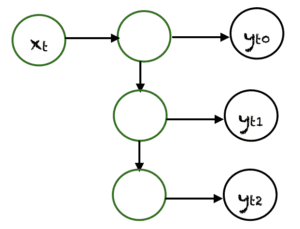
One To Many
One-to-Many is a type of RNN that gives multiple outputs when given a single input. It takes a fixed input size and gives a sequence of data outputs. Its models can be applied to music generation and image captioning.
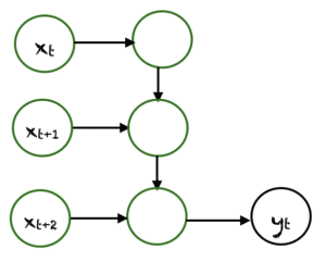
Many To One
Many-to-One is used when a single output is required from multiple input units or a sequence of them. It takes a sequence of inputs to display a fixed output. Sentiment analysis is a common example of this type of recurrent neural network.
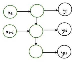
Many To Many
Many-to-Many is used to generate a sequence of output data from a sequence of input units. This type of RNN is divided into two subcategories:
1. Equal size of units: In this case, the number of input and output units is the same. A common application can be found in Name-Entity Recognition.

2. Unequal size of units: In this case, the inputs and outputs have a different number of units. Its application can be found in machine translation.
Limitations and variants of RNNs
Recurrent neural networks suffer from a problem called gradient disappearance, which is also a common problem for other neural network algorithms. The vanishing gradient problem is the result of an algorithm called retropropagation which allows neural networks to optimize the learning process.
In short, the neural network model compares the difference between its output and the desired output and feeds this information back to the network to adjust parameters such as weights using a value called a gradient. A larger gradient value implies larger parameter adjustments, and vice versa. This process continues until a satisfactory level of accuracy is achieved.
RNNs exploit the backpropagation over time (BPTT) algorithm where the calculations depend on the previous steps. However, if the gradient value is too small in a step during the backconversion, the value will be even smaller in the next step. This causes the gradients to decrease exponentially to a point where the model stops learning.
This is called the vanishing gradient problem and causes RNNs to have short-term memory: past outputs increasingly have little or no effect on current output.
The leakage gradient problem can be solved by different variants of RNNs. Two of them are:
- LSTM (called Long Short-Term Memory): They are able to remember entries over a long period of time. This is because they hold information in memory, much like computer memory. The LSTM can read, write and delete information from its memory. In this memory, one decides each time to store or to delete information according to the importance which it grants to information. The assignment of importance is done by weights, which are also learned by the algorithm.
- GRU (Gated Recurrent Units): This model is similar to LSTM because it also solves the short-term memory problem of RNN models. To solve this problem, GRU integrates the two gate operation mechanisms called Update gate and Reset gate: the reset and update gates are concretely vectors that control what information to keep and what to discard.
Recurrent neural networks are a versatile tool that can be used in a variety of situations. They are employed in various linguistic modeling and text generation methods. They are also used in voice recognition. However, they have one flaw. They are slow to train and have difficulty learning long-term addictions.
