
In the fascinating and intricate world of investments, one metric stands out as a universal benchmark for evaluating the performance of an investment or a portfolio: the Sharpe Ratio. Named after William F. Sharpe, a Nobel Laureate in Economic Sciences, this ratio allows investors and fund managers to measure the risk-adjusted return of an investment. In other words, it tells us how much return we can expect for the level of risk we are taking. How to build a Sharpe ratio calculator?
This ratio is critically important, as all investments come with some degree of risk. Yet, not all risk is rewarded equally. By using the Sharpe Ratio, investors can compare and contrast different investment opportunities, striking a balance between risk and reward.
In this article, we’re going to delve deeper into the concept of the Sharpe Ratio, understand its significance, and learn how to calculate it in three different ways using Python, a popular programming language in the field of finance and data analysis. Whether you’re an experienced investor, a budding financial analyst, or a coding enthusiast, this article will equip you with the knowledge and practical skills to quantify investment performance and make informed decisions. Get ready to add a powerful tool to your investment analysis toolkit.
The Sharpe Ratio Formula
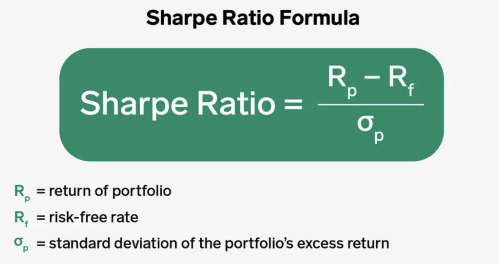
The Sharpe Ratio is a measure for calculating risk-adjusted return, and its formula is as follows:
Sharpe Ratio = (Rp – Rf) / σp
where,
- Rp is the expected return of the portfolio
- Rf is the risk-free rate
- σp is the standard deviation of the portfolio’s excess return
This formula calculates the difference between the returns of the investment and the risk-free return, per unit of volatility.
The risk-free rate is the return that can be obtained with zero risk, usually taken as the yield on a U.S. government bond, such as a 3-month or 10-year Treasury bill. The portfolio’s return is the return obtained from the portfolio (or investment), and the standard deviation of the portfolio’s return is a measure of the investment’s volatility.
The resulting ratio is a measure of risk-adjusted performance. A higher Sharpe Ratio indicates that the risk taken on the investment is more adequately rewarded with higher returns, whereas a lower Sharpe Ratio indicates that the returns are not justified by the risk taken.
Implement a Sharpe Ratio Calculator in Python
Here’s a simple snippet of code for calculating the Sharpe Ratio using Python:
import numpy as np
import pandas as pd

# Assuming you have a DataFrame 'df' with daily returns for your portfolio and the risk-free rate
df = pd.DataFrame({
    'portfolio': [0.01, 0.02, -0.01, -0.02, 0.01, 0.02, -0.01, -0.02, 0.01, 0.02],
    'risk_free': [0.001, 0.001, 0.001, 0.001, 0.001, 0.001, 0.001, 0.001, 0.001, 0.001]
})

# Calculate excess returns
df['excess_return'] = df['portfolio'] - df['risk_free']

# Calculate the Sharpe Ratio
sharpe_ratio = np.mean(df['excess_return']) / np.std(df['excess_return'])

# Annualize the Sharpe Ratio
annual_factor = np.sqrt(252)  # Use 252 for daily returns, 52 for weekly returns, 12 for monthly returns
sharpe_ratio_annualized = sharpe_ratio * annual_factor

print('Sharpe Ratio (Annualized):', sharpe_ratio_annualized)
In this Sharpe ratio calculator example, we first calculate the excess returns by subtracting the risk-free rate from the portfolio returns. We then calculate the Sharpe Ratio as the mean of the excess returns divided by the standard deviation of the excess returns. We also annualize the Sharpe Ratio assuming 252 trading days in a year.
Keep in mind that you’ll need to replace the sample data in this snippet with your own actual data. Also, the time period you’re using (daily, weekly, monthly, etc.) will affect your calculations. Adjust the annual factor accordingly based on the frequency of your data.
Calculate the Efficient Frontier
In modern portfolio theory, the efficient frontier is a set of optimal portfolios that offer the highest expected return for a defined level of risk or the lowest risk for a given level of expected return. Portfolios that lie below the efficient frontier are sub-optimal, because they do not provide enough return for the level of risk. Portfolios that cluster to the right of the efficient frontier are also sub-optimal, because they have a higher level of risk for the defined rate of return.
In Python, we can use the PyPortfolioOpt library to compute the efficient frontier. Below is a simple example of how you can do this:
import numpy as np
import pandas as pd
from pypfopt import EfficientFrontier
from pypfopt import risk_models
from pypfopt import expected_returns

# Sample price data
data = pd.DataFrame({
    'Asset1': np.random.normal(1.01, 0.03, 100),
    'Asset2': np.random.normal(1.02, 0.05, 100),
    'Asset3': np.random.normal(1.03, 0.07, 100),
})

# Calculate expected returns and the covariance matrix of returns
mu = expected_returns.mean_historical_return(data)
S = risk_models.sample_cov(data)

# Optimize for maximal Sharpe ratio
ef = EfficientFrontier(mu, S)
weights = ef.max_sharpe()

cleaned_weights = ef.clean_weights()
ef.portfolio_performance(verbose=True)
Conclusion
In conclusion, understanding and effectively calculating the Sharpe Ratio, as well as comprehending the concept of the Efficient Frontier, are crucial skills for any investor or financial analyst. These techniques provide a quantitative basis to measure the risk-adjusted returns of an investment or a portfolio.
The Sharpe Ratio measures how much excess return you are receiving for the extra volatility that you endure for holding a riskier asset. A higher Sharpe Ratio could potentially indicate a more favorable risk/return trade-off.
On the other hand, the Efficient Frontier helps to identify the optimal portfolios that offer the highest expected return for a defined level of risk. By plotting different portfolios on a graph with expected return on the y-axis and standard deviation (or volatility) on the x-axis, the Efficient Frontier illustrates the limit of possible portfolio allocations.
Python, as we’ve seen, provides robust and efficient tools to carry out these calculations. Libraries such as pandas, numpy, and PyPortfolioOpt simplify these tasks, enabling even those new to the field of finance to perform complex financial analyses.
However, while these tools are powerful, it’s important to remember that they’re based on historical data and certain assumptions, and therefore cannot guarantee future performance. They should be used as part of a broader toolkit when making investment decisions.
Remember, successful investing is not just about computation but also about interpretation and understanding the bigger picture.
n.b: this is not financial advice
